Solving Data Mysteries with Plots
This post will expand on the topic of data plotting which was discussed in this post, https://www.cloudacm.com/?p=4136. The concept is to give a quick at a glance view of information. Details can be lost in lengthy data sets formatted in tables or flat files, which are tedious to sift through. Data fatigue is problem for those not prepared to handle large amounts of information. The apathy it can foster can turn a resource into a liability. By using plots, it’s the hope that the fatigue can be reduced.
Below are plot examples. Some of these plots were originally intended to represent data of a given nature. However, the limitations became clear and this led to other plot methods being used. Those details will be covered in the following examples.
Interpolated Heat-map Plots
This was a fundamental plot that was covered in the earlier post. It fills in missing data points from the available data. Details can be found here, https://docs.astropy.org/en/stable/convolution/index.html. The limitation of this type of plot is that the sparsely available data points should be evenly distributed across the array. Using data sets that are grouped on one region of the array would result in a plot that poorly represents the entire array.
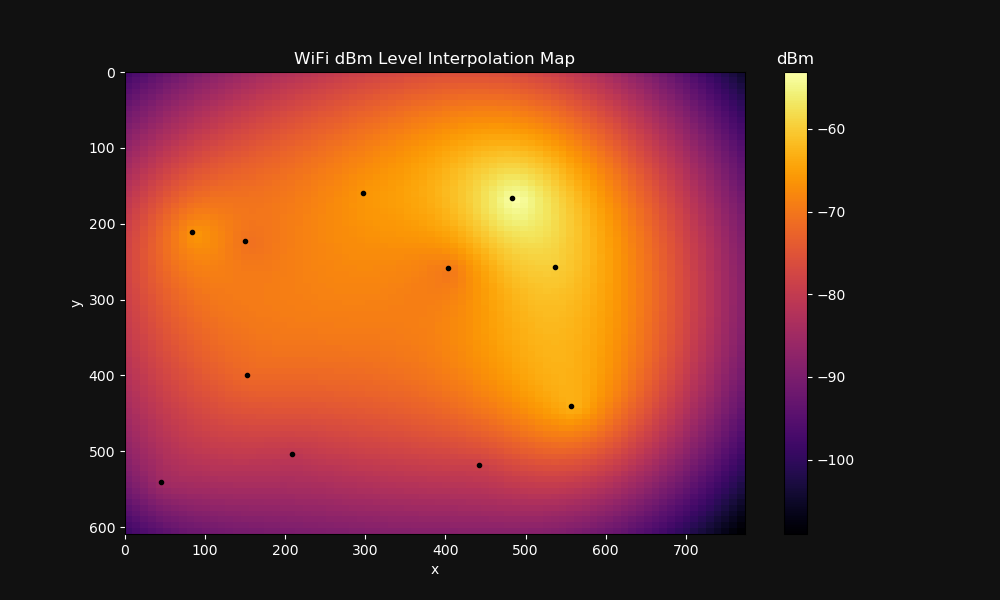
The plot was created from this data set file called “Heatmap.csv”. Here is the content of that file.
x,y,dBm
84,211,-66
45,541,-85
150,223,-71
152,400,-72
208,504,-81
297,160,-66
403,259,-70
442,518,-79
483,166,-53
537,257,-60
557,440,-63
The python script used to create the plot image is as follows.
import matplotlib.pyplot as plt
import numpy as np
from scipy.interpolate import Rbf  # radial basis functions
import pandas as pd

# Create the figure with a colored background
fig = plt.figure(facecolor='#111111')

# Read the CSV file
df = pd.read_csv('Heatmap.csv')

# Extract the columns into arrays
x = df['x'].values
y = df['y'].values
z = df['dBm'].values

# RBF Func
rbf_fun = Rbf(x, y, z, function='linear')

x_new = np.linspace(0, 774, 81)
y_new = np.linspace(0, 609, 82)

x_grid, y_grid = np.meshgrid(x_new, y_new)
z_new = rbf_fun(x_grid.ravel(), y_grid.ravel()).reshape(x_grid.shape)

# Create the plot with a black background
plt.pcolor(x_new, y_new, z_new, cmap=plt.cm.inferno)
plt.plot(x, y, '.', color='black')
# Marker styles - https://matplotlib.org/stable/api/markers_api.html

# Flip the y-axis
plt.gca().invert_yaxis()

# Set the text and labels to white
plt.xlabel('x', color='white')
plt.ylabel('y', color='white')
plt.title('WiFi dBm Level Interpolation Map', color='white')

# Set the tick labels to white
plt.gca().tick_params(axis='x', colors='white')
plt.gca().tick_params(axis='y', colors='white')

# Set the colorbar tick labels to white
cbar = plt.colorbar()
cbar.ax.set_title('dBm', color='white')
cbar.ax.yaxis.set_tick_params(color='white')
plt.setp(plt.getp(cbar.ax.axes, 'yticklabels'), color='white')

# Scale the plot
F = plt.gcf()
Size = F.get_size_inches()
F.set_size_inches(10, 6)

# Show the plot
# plt.show()

# Save the plot to an image file
plt.savefig('Heatmap_rev2.png', facecolor=fig.get_facecolor())
X Y Scatter Map Plots
This plot addresses the issue of data set grouping. The data is clearly presented, whereas an interpolated heat-map would misrepresent the data. This plot method lends itself well to data collection that isn’t sparsely distributed. Data collection along a linear path is easier to understand.
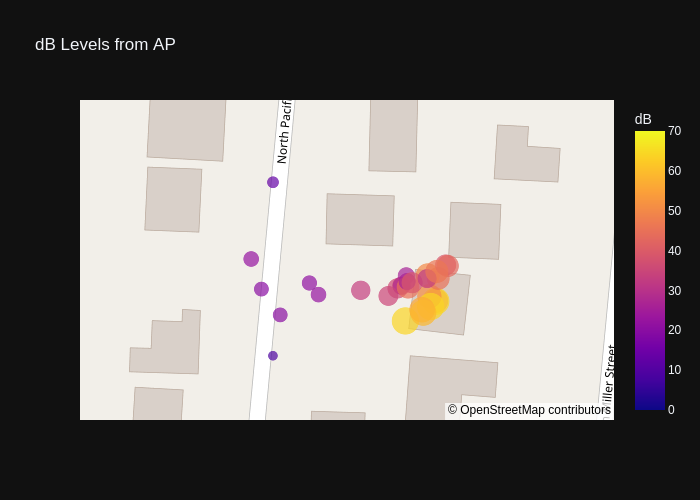
The “dB Levels from AP” plot was created from this data set file called “Walk 1 Modified 1.csv”. Here is the content of that file.
latitude,longitude,dB
45.6230045250113,-123.943566307541,51
45.623003686821,-123.943566726636,64
45.6230130058772,-123.943584069679,51
45.6230464727475,-123.943560211466,45
45.6230522372454,-123.943588495543,50
45.6230514542379,-123.943646113292,26
45.6230331887133,-123.943659706114,28
45.6230278109592,-123.943669336702,36
45.6230324078192,-123.943658347377,29
45.623013621687,-123.943694105842,35
45.6230161084721,-123.94388152638,22
45.623026389686,-123.944034475971,20
45.6230828880484,-123.944061958182,22
45.6232268704852,-123.944003476674,13
45.6234610491972,-123.943965270902,6
45.6227654362132,-123.944021701665,8
45.6229013909339,-123.944003657099,9
45.622977980632,-123.943984013679,20
45.6230378102009,-123.943905805539,21
45.6230241161965,-123.943767929974,33
45.6230300339537,-123.943641204668,45
45.6230406270525,-123.943643787416,26
45.6230383571552,-123.943630397927,39
45.6230462019293,-123.943590268304,32
45.623071628887,-123.943540407012,39
45.6230697504328,-123.943534749932,43
45.6230595847248,-123.943563926808,46
45.6229937469911,-123.943580520518,64
45.6229876694104,-123.943603757507,56
45.6229820100337,-123.943600383094,59
45.622966645897,-123.943648465306,64
The python script used to create the plot image is as follows.
# See, https://stackabuse.com/plotly-scatter-plot-tutorial-with-examples/

import pandas as pd
import plotly.express as px


df = pd.read_csv('Walk 1 Modified 1.csv')

fig = px.scatter_mapbox(df,
    lat = 'latitude',
    lon = 'longitude',
    color = 'dB',
    size = 'dB',
    range_color = (0,70),
    center = dict(lat = 45.623081, lon = -123.943805),
    zoom = 18,
    mapbox_style = 'open-street-map',
    title = 'dB Levels from AP',
    template='plotly_dark' )


fig.write_image("Heatmap_example4.png")
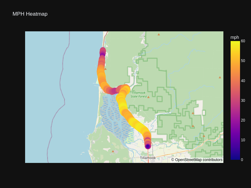
The “MPH Heatmap” plot was created from this data set file called “Drive 1 MPH.csv”. The data is available here for download, Drive 1 MPH
The python script used to create the plot image is as follows.
# See, https://stackabuse.com/plotly-scatter-plot-tutorial-with-examples/

import pandas as pd
import plotly.express as px


df = pd.read_csv('Drive 1 MPH.csv')

fig = px.scatter_mapbox(df,
    lat = 'latitude',
    lon = 'longitude',
    color = 'mph',
    size = 'mph',
    range_color = (0,60),
    center = dict(lat = 45.549226, lon = -123.896205),
    zoom = 10,
    mapbox_style = 'open-street-map',
    title = 'MPH Heatmap',
    width = 800,
    height = 600,
    template='plotly_dark' )


fig.write_image('Drive 1 MPH Rev 2.png')
X Y Scatter Plots
The method of scatter plots is well suited when merging data values from different sources and scales. This plot shows AP channels at a given point in time and their corresponding power level.
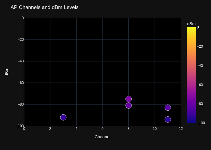
The “AP Channels and dBM Levels” plot was created from a data set file called “Wifi_Readings.csv”. The information contained in this file is confidential and can not be released to the public. It was generated from an ESP32-Cam module that performed a wifi scan and wrote the results to the microSD media. The format of the readings followed this format.
13631,5,SSID-Name-1,-64,AA:BB:CC:DD:EE:FF,1,WPA2
15447,5,SSID-Name-1,-91,BB:CC:DD:EE:FF:AA,6,WPA2
15578,5,SSID-Name-2,-91,CC:DD:EE:FF:AA:BB,11,WPA2
15807,5,*.*Hidden*.*,-91,DD:EE:FF:AA:BB:CC,11,WPA2
15924,5,*.*Hidden*.*,-92,EE:FF:AA:BB:CC:DD,11,WPA2
The following bash script was used to process the csv data set file to allow each scan moment to be plotted, allowing a series of images to be created spanning the entire survey time.
#!/bin/bash
# cloudacm.com
# a shell script to convert ESP32 Wifi Scan Data into dBm Channel Plots.


sed 's/^\s*$/Time in millis,Networks Found,SSID,dBm,AP Mac Address,Channel,Security/' Wifi_Readings.csv > Process-CSV1.tmp

sed -e 's/$/^/g' Process-CSV1.tmp > Process-CSV2.tmp

tr -d '\n' < Process-CSV2.tmp > Process-CSV3.tmp

sed -e 's/Time in millis,/\nTime in millis,/g' Process-CSV3.tmp > Process-CSV4.tmp

split -l 1 Process-CSV4.tmp Process-CSV5_ -a 5 -d


for i in Process-CSV5_*; do
    echo "$i"
    tr "^" "\n" < "$i" > "Re$i"
done

for i in ReProcess-CSV5_*; do
    echo "$i"
    python dBm-Channel-Readings-FileArgument.py "$i"
    # sleep .5
done

exit

#
Here is the python code that is called by the bash script.
import pandas as pd
import plotly.express as px
import sys
import os

path = sys.argv[1]

# Check if the file is empty or has only headers
df = pd.read_csv(path)
if df.empty:
    print(f"Skipping file with no data: {path}")
    sys.exit()

fig = px.scatter(df,
    x='Channel',
    y='dBm',
    color='dBm',
    range_color=(-100,0),
    template='plotly_dark',
    color_continuous_scale='Plasma')

# fig.show()
fig.update_layout(title="AP Channels and dBm Levels",
    xaxis_range=[0,15], yaxis_range=[-100,0],
    paper_bgcolor="#111111", plot_bgcolor='#000000')

fig.update_traces(marker=dict(size=20,
        line=dict(width=1,
        color='silver')),
        selector=dict(mode='markers'))

fig.write_image(f"{(path)}.png")
The plot that follows shows RF levels over a period of time. The time scale of this plot spans the entire time of the data survey.
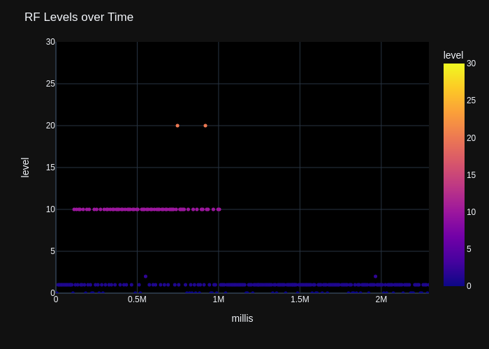
The “RF Levels over Time” plot was created from this data set file called “NRF24L01_PowerReadings.csv”. The data is available here for download, NRF24L01_PowerReadings
The following bash script was used to allow the data set to be passed into the python script as an argument.
#!/bin/bash
# cloudacm.com
# a shell script to plot NRF24Lo1 Power Levels.

python NRF24L01_PowerReadings.py NRF24L01_PowerReadings.csv
sleep 10
exit

#
Here is the python code that is called by the bash script.
import pandas as pd
import plotly.express as px
import sys
import os

path = sys.argv[1]

# Check if the file is empty or has only headers
df = pd.read_csv(path)
if df.empty:
    print(f"Skipping file with no data: {path}")
    sys.exit()

fig = px.scatter(df,
    x='millis',
    y='level',
    color='level',
    range_color=(0,30),
    template='plotly_dark',
    color_continuous_scale='Plasma')

# fig.show()
fig.update_layout(title="RF Levels over Time",
    xaxis_range=[0,2292858], yaxis_range=[0,30],
    paper_bgcolor="#111111", plot_bgcolor='#000000')

fig.update_traces(marker=dict(size=5),
        selector=dict(mode='markers'))

fig.write_image(f"{(path)}.png")
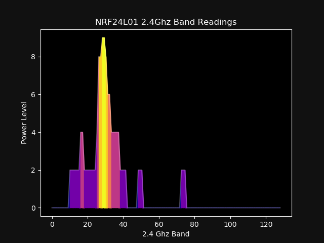
Line-space Plots
This plot is similar to the earlier AP channel plot. But the plot uses a line and area fill that contains a gradient value defined by the power level. The intensity of the larger values are highlighted, giving focus to the observer.
The following bash script was used to process the NRF data set and call the python script for each image.
#!/bin/bash
# cloudacm.com
# a shell script to convert NRF24L01 data into Plots.


split -l 1 NRF24L01_Readings.csv X_Process_NRF-CSV_rev1_ -a 5 -d

for i in X_Process_NRF-CSV_rev1_*; do # Whitespace-safe but not recursive.
    echo "$i"
    python Process_NRF-CSV_rev1.py "$i"
    # sleep .5
done

exit

#
Here is the python script that the bash script calls.
import matplotlib.pyplot as plt
import numpy as np
# Uncomment for a custom colormap
# from matplotlib.colors import LinearSegmentedColormap
import csv
import sys

path = sys.argv[1]

# Read data from readings.csv
with open((path), 'r') as file:
    reader = csv.reader(file)
    y = list(map(int, next(reader)))

# Generate x values
x = np.linspace(0, len(y), len(y))

# Create a custom colormap
# cmap = LinearSegmentedColormap.from_list('gradient', ['red', 'yellow'])
cmap = plt.cm.get_cmap('plasma')

# Create the plot
fig, ax = plt.subplots()
fig.patch.set_facecolor('#111111')
ax.set_facecolor('black')
ax.spines['bottom'].set_color('white')
ax.spines['top'].set_color('white')
ax.spines['right'].set_color('white')
ax.spines['left'].set_color('white')
ax.xaxis.label.set_color('white')
ax.yaxis.label.set_color('white')
ax.title.set_color('white')
ax.tick_params(axis='x', colors='white')
ax.tick_params(axis='y', colors='white')
line = ax.plot(x, y, label='Data Line', color='white', alpha=0.25)

# Fill the area underneath the line with a vertical gradient
for i in range(len(x)-1):
    ax.fill_between(x[i:i+2], y[i:i+2], color=cmap(y[i]/max(y)), alpha=1)

# Add labels and title
plt.xlabel('2.4 Ghz Band')
plt.ylabel('Power Level')
plt.title('NRF24L01 2.4Ghz Band Readings')

# Show the plot
# plt.show()
plt.savefig(f"{(path)}", facecolor=fig.get_facecolor())
Here is the data set from the NRF24L01 which was captured using an ESP32-Cam module to the microSD media, NRF24L01_Readings
Polar Plots
The polar plot is ideal when data is gathered from a given direction. This gives a top down view of the data collection occurring at the center point. The source can be located using this method.
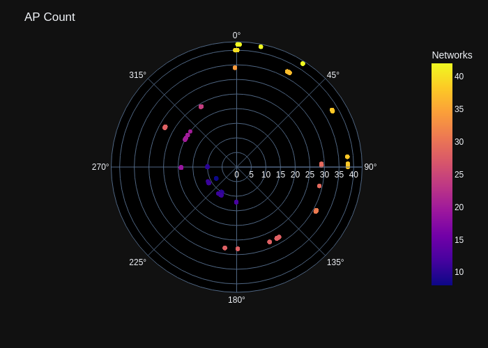
This is the python script used to create the plot. The data set is available here for download, Sample-1_Networks_Readings
import pandas as pd
import plotly.express as px

df = pd.read_csv('Sample-1_Networks_Readings.csv')
fig = px.scatter_polar(df,
         r="Networks",
         theta="Heading",
         color="Networks",
         template='plotly_dark',
         color_continuous_scale='Plasma')

fig.update_layout(title="AP Count",
    paper_bgcolor="#111111")

fig.update_polars(bgcolor='#000000')

fig.write_image('Sample-1_Networks_Readings-rev4.png')


# See https://plotly.com/python/colorscales/
# or https://plotly.com/python/builtin-colorscales/
# color_continuous_scale='viridis'
# color_continuous_scale='viridis_r'
# color_continuous_scale='plasma_r'
# color_continuous_scale='ice'
# color_continuous_scale=["red", "green", "blue"]
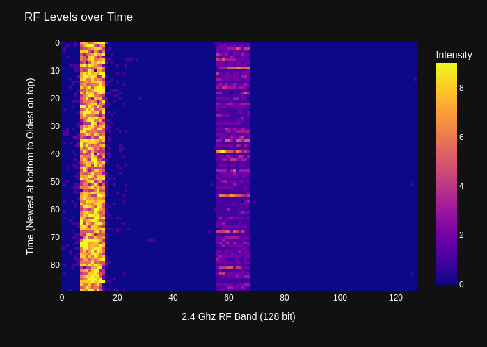
Waterfall Plots
These plots are time based, typically with recent readings at the bottom of the plot window. Fast Fourier transform data is often represented with a waterfall plot to show deviation over time.
Here is the bash script used to call the python script.
#!/bin/bash
# cloudacm.com
# a shell script to convert NRF24L01 Data into waterfall Plots.

python NRF24L01_Waterfall.py

exit

#
This is the python code used to plot each instance of the NRF24L01 data with some blank buffering at the beginning. The data set can be downloaded here, NRF24L01_Readings
import sys, os
import plotly.express as px
from numpy import genfromtxt

# Read the CSV file to get the total number of rows
with open('NRF24L01_Readings.csv', 'r') as file:
    total_rows = sum(1 for row in file)

# Define the max_rows value
max_rows = 90

# Initialize skip_header value
skip_header = 0

while skip_header <= total_rows - max_rows:
    # Read the data with the current skip_header value
    numpy_array = genfromtxt(
        'NRF24L01_Readings.csv',
        delimiter=',',
        skip_header=skip_header,
        max_rows=max_rows
    )

    # Create the plot
    fig = px.imshow(numpy_array, color_continuous_scale='plasma')

    fig.update_layout(
        title="RF Levels over Time",
        paper_bgcolor="#111111",
        coloraxis_colorbar=dict(title="Intensity"),
        font=dict(color="white")
    )

    fig.update_xaxes(
        showticklabels=True,
        title_text="2.4 Ghz RF Band (128 bit)",
        tickfont=dict(color="white")
    ).update_yaxes(
        showticklabels=True,
        title_text="Time (Newest at bottom to Oldest on top)",
        tickfont=dict(color="white")
    )

    # Save the image with the skip_header value in the filename
    fig.write_image(f"NRF24L01_Waterfall_skip_{skip_header}.png")

    # Increment the skip_header value by 1
    skip_header += 1
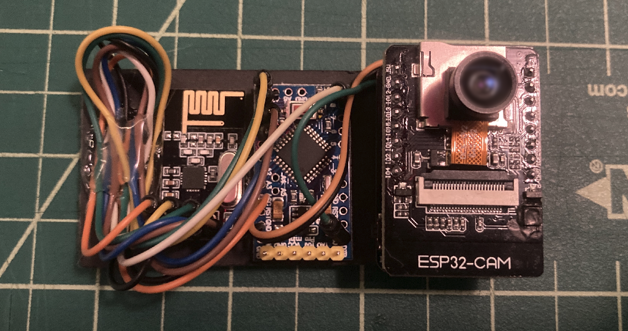
The data in these plots were captured using an ESP32-Cam module, Arduino Pro Mini, and/or NRF24L01 module. Data was also captured in tandem using the iPhone app SensorLog. Here is a link to the app. The app can be used on iPads and the Apple Watch.
Here is the code used for the stand alone ESP32-Cam module to survey WiFi Networks.
/*
 *  This sketch demonstrates how to scan WiFi networks.
 *  The API is based on the Arduino WiFi Shield library, but has significant changes as newer WiFi functions are supported.
 *  E.g. the return value of `encryptionType()` different because more modern encryption is supported.
 */
#include "WiFi.h"
#include "FS.h"                // SD Card ESP32
#include "SD_MMC.h"            // SD Card ESP32
const char* WifiScanReadings = "/Wifi-Scan_Readings.csv";

void HardwareSetup()
{
    // Set WiFi to station mode and disconnect from an AP if it was previously connected.
    WiFi.mode(WIFI_STA);
    WiFi.disconnect();
    delay(100);
}

void PrintHeader()
{
   appendFile(SD_MMC, WifiScanReadings, "ESP32-Cam-Wifi-Scan-MicroSD_Ver3");
   appendFile(SD_MMC, WifiScanReadings, "\n");
   appendFile(SD_MMC, WifiScanReadings, "Time in millis,Networks Found,SSID,dBm,AP Mac Address,Channel,Security");
   appendFile(SD_MMC, WifiScanReadings, "\n");
   appendFile(SD_MMC, WifiScanReadings, "\n");
}

void StartupMicroSD() {
  if(!SD_MMC.begin()){
    return;
  }
  uint8_t cardType = SD_MMC.cardType();
  if(cardType == CARD_NONE){
    return;
  }
}


//Append to the end of file in SD card
void appendFile(fs::FS &fs, const char * path, const char * message){

    File file = fs.open(path, FILE_APPEND);
    if(!file){
        return;
    }
    if(file.print(message)){
    } else {
    }
}


void ScanWifiNetworks()
{
      // WiFi.scanNetworks will return the number of networks found.
    int IntWifiNetworks = WiFi.scanNetworks(/*async=*/false, /*hidden=*/true);

    if (IntWifiNetworks == 0) {
    }

    else {

        for (int NetworkCount = 0; NetworkCount < IntWifiNetworks; ++NetworkCount)
           {

            String MillisString = String(millis());         // read string until meet newline character
            appendFile(SD_MMC, WifiScanReadings, MillisString.c_str());
            appendFile(SD_MMC, WifiScanReadings, ",");

            String StringWifiNetworks = String(IntWifiNetworks);         // read string until meet newline character
            appendFile(SD_MMC, WifiScanReadings, StringWifiNetworks.c_str());
            appendFile(SD_MMC, WifiScanReadings, ",");

            String StringSSID = String(WiFi.SSID(NetworkCount));
            if(StringSSID != NULL) {
              appendFile(SD_MMC, WifiScanReadings, StringSSID.c_str());
              }
            else {
              appendFile(SD_MMC, WifiScanReadings, "*.*Hidden*.*");
              }
            appendFile(SD_MMC, WifiScanReadings, ",");

            String StringRSSI = String(WiFi.RSSI(NetworkCount));
            appendFile(SD_MMC, WifiScanReadings, StringRSSI.c_str());
            appendFile(SD_MMC, WifiScanReadings, ",");

            String StringBSSIDstr = String(WiFi.BSSIDstr(NetworkCount));
            appendFile(SD_MMC, WifiScanReadings, StringBSSIDstr.c_str());
            appendFile(SD_MMC, WifiScanReadings, ",");


            String StringChannel = String(WiFi.channel(NetworkCount));
            appendFile(SD_MMC, WifiScanReadings, StringChannel.c_str());
            appendFile(SD_MMC, WifiScanReadings, ",");

            printEncryptionType(WiFi.encryptionType(NetworkCount));
            appendFile(SD_MMC, WifiScanReadings, "\n");
           }
       }

      // Delete the scan result to free memory for code below.
      WiFi.scanDelete();
}


void printEncryptionType(int thisType) {

  // read the encryption type and print out the name:
  switch (thisType) {
            case WIFI_AUTH_OPEN:
                appendFile(SD_MMC, WifiScanReadings, "open");
                break;
            case WIFI_AUTH_WEP:
                appendFile(SD_MMC, WifiScanReadings, "WEP");
                break;
            case WIFI_AUTH_WPA_PSK:
                appendFile(SD_MMC, WifiScanReadings, "WPA");
                break;
            case WIFI_AUTH_WPA2_PSK:
                appendFile(SD_MMC, WifiScanReadings, "WPA2");
                break;
            case WIFI_AUTH_WPA_WPA2_PSK:
                appendFile(SD_MMC, WifiScanReadings, "WPA+WPA2");
                break;
            case WIFI_AUTH_WPA2_ENTERPRISE:
                appendFile(SD_MMC, WifiScanReadings, "WPA2-EAP");
                break;
            case WIFI_AUTH_WPA3_PSK:
                appendFile(SD_MMC, WifiScanReadings, "WPA3");
                break;
            case WIFI_AUTH_WPA2_WPA3_PSK:
                appendFile(SD_MMC, WifiScanReadings, "WPA2+WPA3");
                break;
            case WIFI_AUTH_WAPI_PSK:
                appendFile(SD_MMC, WifiScanReadings, "WAPI");
                break;
            default:
                appendFile(SD_MMC, WifiScanReadings, "unknown");
  }
}


void setup() {
  StartupMicroSD();
  HardwareSetup();
  PrintHeader();

  // Let things settle before logging
  delay(1000);
}


void loop() {
  // This can take 12 seconds to complete
  ScanWifiNetworks();
  appendFile(SD_MMC, WifiScanReadings, "\n");
}
The following code is in two parts, the first is the Arduino Pro Mini code that interfaces with the NRF24L01 and provides a serial stream to the ESP32-Cam module. The second part is the ESP-32 Cam module code that listens for the serial stream from the Pro Mini and then performs a wifi scan once the stream is finished, all data is then written to the microSD media. Oh yeah, I almost forgot to mention that it also takes a photo and saves the image file.
#include <SPI.h>

// Increased define CHANNELS from 64 to 256 in attempt to increase resolution

// Poor Man's Wireless 2.4GHz Scanner
// See, https://forum.arduino.cc/t/poor-mans-2-4-ghz-scanner/54846
//
// uses an nRF24L01p connected to an Arduino
//
// Cables are:
//     SS       -> 10   Chip Select Not - This is held to VCC to turn on chip, GPIO is not needed
//     MOSI     -> 11   Master Out Slave In - Now called PICO
//     MISO     -> 12   Master In Slave Out - Now called POCI
//     SCK      -> 13   Clock Signal
//
//     GND and VCC sould have a 10uf capacitor between them
//
// and CE       ->  9   Chip Enable - This is needed because SPI requires 2 way comms
//
// created March 2011 by Rolf Henkel
//

#define CE  9  // Chip Enable - This is needed because SPI requires 2 way comms

unsigned long myTime;

// Array to hold Channel data (32 = 1 sec, 64 = 2 sec, 128 = 4 sec, 256 = 8 sec, etc)
#define CHANNELS 128
int channel[CHANNELS];

// greyscale mapping
int  line;
char grey[] = "0123456789";
// char grey[] = " .:-=+*aRW";

// nRF24L01P registers we need
#define _NRF24_CONFIG      0x00
#define _NRF24_EN_AA       0x01
#define _NRF24_RF_CH       0x05
#define _NRF24_RF_SETUP    0x06
#define _NRF24_RPD         0x09

// get the value of a nRF24L01p register
byte getRegister(byte r)
{
  byte c;

  PORTB &=~_BV(2);
  c = SPI.transfer(r&0x1F);
  c = SPI.transfer(0);
  PORTB |= _BV(2);

  return(c);
}

// set the value of a nRF24L01p register
void setRegister(byte r, byte v)
{
  PORTB &=~_BV(2);
  SPI.transfer((r&0x1F)|0x20);
  SPI.transfer(v);
  PORTB |= _BV(2);
}

// power up the nRF24L01p chip
void powerUp(void)
{
  setRegister(_NRF24_CONFIG,getRegister(_NRF24_CONFIG)|0x02);
  delayMicroseconds(130);
}

// switch nRF24L01p off
void powerDown(void)
{
  setRegister(_NRF24_CONFIG,getRegister(_NRF24_CONFIG)&~0x02);
}

// enable RX
void enable(void)
{
    PORTB |= _BV(1);
}

// disable RX
void disable(void)
{
    PORTB &=~_BV(1);
}

// setup RX-Mode of nRF24L01p
void setRX(void)
{
  setRegister(_NRF24_CONFIG,getRegister(_NRF24_CONFIG)|0x01);
  enable();
  // this is slightly shorter than
  // the recommended delay of 130 usec
  // - but it works for me and speeds things up a little...
  delayMicroseconds(100);
}

// scanning all channels in the 2.4GHz band
void scanChannels(void)
{
  disable();
  for( int j=0 ; j<200  ; j++)
  {
    for( int i=0 ; i<CHANNELS ; i++)
    {
      // select a new channel
      setRegister(_NRF24_RF_CH,(128*i)/CHANNELS);

      // switch on RX
      setRX();

      // wait enough for RX-things to settle
      delayMicroseconds(40);

      // this is actually the point where the RPD-flag
      // is set, when CE goes low
      disable();

      // read out RPD flag; set to 1 if
      // received power > -64dBm
      if( getRegister(_NRF24_RPD)>0 )   channel[i]++;
    }
  }
}

// outputs channel data as a simple grey map
void outputChannels(void)
{
  int norm = 0;

  // find the maximal count in channel array
  for( int i=0 ; i<CHANNELS ; i++)
    if( channel[i]>norm ) norm = channel[i];

  // now output the data
  for( int i=0 ; i<CHANNELS ; i++)
  {
    int pos;

    // calculate grey value position
    if( norm!=0 ) pos = (channel[i]*10)/norm;
    else          pos = 0;

    // boost low values
    if( pos==0 && channel[i]>0 ) pos++;

    // clamp large values
    if( pos>9 ) pos = 9;

    // print it out
    Serial.print(grey[pos]);
    Serial.print(',');
    channel[i] = 0;
  }

  // indicate overall power
  Serial.print(norm);
  Serial.print(',');
  myTime = millis();
  Serial.print(myTime);
  Serial.println(',');
}


void setup()
{
  Serial.begin(115200);

  // Setup SPI
  SPI.begin();
  // Clock Speed, Bit Order, and Data Mode
  SPI.beginTransaction(SPISettings(20000000, MSBFIRST, SPI_MODE0));

  // Activate Chip Enable
  pinMode(CE,OUTPUT);
  disable();

  // now start receiver
  powerUp();

  // switch off Shockburst
  setRegister(_NRF24_EN_AA,0x0);

  // make sure RF-section is set properly
  // - just write default value...
  setRegister(_NRF24_RF_SETUP,0x0F);

  // reset line counter
  line = 0;
}

void loop()
{
  // do the scan
  scanChannels();

  Serial.print('#');
  Serial.print(',');

  // output the result
  outputChannels();
}
/*********
  Rui Santos
  Complete project details at https://RandomNerdTutorials.com/esp32-cam-take-photo-save-microsd-card

  IMPORTANT!!!
   - Select Board "AI Thinker ESP32-CAM"
   - GPIO 0 must be connected to GND to upload a sketch
   - After connecting GPIO 0 to GND, press the ESP32-CAM on-board RESET button to put your board in flashing mode

  Permission is hereby granted, free of charge, to any person obtaining a copy
  of this software and associated documentation files.
  The above copyright notice and this permission notice shall be included in all
  copies or substantial portions of the Software.

*********/

#include "WiFi.h"
#include "esp_camera.h"
#include "FS.h"                // SD Card ESP32
#include "SD_MMC.h"            // SD Card ESP32
const char* NRFReadings = "/NRF24L01_Readings.csv";
const char* WifiScanReadings = "/Wifi_Readings.csv";
String MillisString;


// Pin definition for CAMERA_MODEL_AI_THINKER
#define PWDN_GPIO_NUM     32
#define RESET_GPIO_NUM    -1
#define XCLK_GPIO_NUM      0
#define SIOD_GPIO_NUM     26
#define SIOC_GPIO_NUM     27
#define Y9_GPIO_NUM       35
#define Y8_GPIO_NUM       34
#define Y7_GPIO_NUM       39
#define Y6_GPIO_NUM       36
#define Y5_GPIO_NUM       21
#define Y4_GPIO_NUM       19
#define Y3_GPIO_NUM       18
#define Y2_GPIO_NUM        5
#define VSYNC_GPIO_NUM    25
#define HREF_GPIO_NUM     23
#define PCLK_GPIO_NUM     22

unsigned long pictureNumber = 0;
unsigned long photodelay = 0; // Time counter for timed photos
unsigned long delaytime = 3000; // Time of delay

unsigned long ExecuteInterval = 2000;
unsigned long LastInterval = 0;
unsigned long CurrentInterval = 0;
int HoldInterval = 0;

void HardwareSetup()
{
  // Note the format for setting a serial port is as follows:
  // Serial.begin(baud-rate, protocol, RX pin, TX pin);
  // initialize serial:
  Serial.begin(115200);
  delay(100);

}


void PrintHeader()
{

   appendFile(SD_MMC, WifiScanReadings, "ESP32-Cam-NRF24L01-Scan-Wifi-Scan-Take-Photo-Save-MicroSD_Ver4");
   appendFile(SD_MMC, WifiScanReadings, "\n");
   appendFile(SD_MMC, WifiScanReadings, "Arduino Pro Mini Firmware - Arduino_ProMini_NRF24L01-128bit-Ver1.ino");
   appendFile(SD_MMC, WifiScanReadings, "\n");
   appendFile(SD_MMC, WifiScanReadings, "Time in millis,Networks Found,SSID,dBm,AP Mac Address,Channel,Security");
   appendFile(SD_MMC, WifiScanReadings, "\n");
   appendFile(SD_MMC, WifiScanReadings, "\n");


}


void StartupCamera() {

  camera_config_t config;
  config.ledc_channel = LEDC_CHANNEL_0;
  config.ledc_timer = LEDC_TIMER_0;
  config.pin_d0 = Y2_GPIO_NUM;
  config.pin_d1 = Y3_GPIO_NUM;
  config.pin_d2 = Y4_GPIO_NUM;
  config.pin_d3 = Y5_GPIO_NUM;
  config.pin_d4 = Y6_GPIO_NUM;
  config.pin_d5 = Y7_GPIO_NUM;
  config.pin_d6 = Y8_GPIO_NUM;
  config.pin_d7 = Y9_GPIO_NUM;
  config.pin_xclk = XCLK_GPIO_NUM;
  config.pin_pclk = PCLK_GPIO_NUM;
  config.pin_vsync = VSYNC_GPIO_NUM;
  config.pin_href = HREF_GPIO_NUM;
  config.pin_sscb_sda = SIOD_GPIO_NUM;
  config.pin_sscb_scl = SIOC_GPIO_NUM;
  config.pin_pwdn = PWDN_GPIO_NUM;
  config.pin_reset = RESET_GPIO_NUM;
  config.xclk_freq_hz = 20000000;
  config.pixel_format = PIXFORMAT_JPEG;  //YUV422,GRAYSCALE,RGB565,JPEG
  config.frame_size = FRAMESIZE_XGA; // FRAMESIZE_ + QVGA (320 x 240) | CIF (352 x 288) |VGA (640 x 480) | SVGA (800 x 600) |XGA (1024 x 768) |SXGA (1280 x 1024) |UXGA (1600 x 1200)
  config.jpeg_quality = 10; // 10-63 lower number means higher quality
  config.fb_count = 1;

  // Init Camera
  esp_err_t err = esp_camera_init(&config);
  if (err != ESP_OK) {
    return;
  }

  sensor_t * s = esp_camera_sensor_get();
  s->set_whitebal(s, 0);       // 0 = disable , 1 = enable
  s->set_awb_gain(s, 0);       // 0 = disable , 1 = enable

}


void StartupMicroSD() {

  if(!SD_MMC.begin()){
    return;
  }

  uint8_t cardType = SD_MMC.cardType();
  if(cardType == CARD_NONE){
    return;
  }

}


//Append to the end of file in SD card
void appendFile(fs::FS &fs, const char * path, const char * message){

    File file = fs.open(path, FILE_APPEND);
    if(!file){
        return;
    }
    if(file.print(message)){
    } else {
    }
}


// https://mischianti.org/esp32-practical-power-saving-manage-wifi-and-cpu-1/


void disableWiFi(){

  // Switch WiFi off
  WiFi.mode(WIFI_OFF);    // Switch WiFi off
  delay(100);
}


void enableWiFi(){

  // Set WiFi to station mode and disconnect from an AP if it was previously connected.
  WiFi.mode(WIFI_STA);
  WiFi.disconnect();
  delay(100);
}


void ScanWifiNetworks()
{

      // WiFi.scanNetworks will return the number of networks found.
    int IntWifiNetworks = WiFi.scanNetworks(/*async=*/false, /*hidden=*/true);


    if (IntWifiNetworks == 0) {
    }

    else {

        for (int NetworkCount = 0; NetworkCount < IntWifiNetworks; ++NetworkCount)
           {

            MillisString = String(millis());         // read string until meet newline character
            appendFile(SD_MMC, WifiScanReadings, MillisString.c_str());
            appendFile(SD_MMC, WifiScanReadings, ",");

            String StringWifiNetworks = String(IntWifiNetworks);         // read string until meet newline character
            appendFile(SD_MMC, WifiScanReadings, StringWifiNetworks.c_str());
            appendFile(SD_MMC, WifiScanReadings, ",");

            String StringSSID = String(WiFi.SSID(NetworkCount));
            if(StringSSID != NULL) {
              appendFile(SD_MMC, WifiScanReadings, StringSSID.c_str());
              }
            else {
              appendFile(SD_MMC, WifiScanReadings, "*.*Hidden*.*");
              }
            appendFile(SD_MMC, WifiScanReadings, ",");

            String StringRSSI = String(WiFi.RSSI(NetworkCount));
            appendFile(SD_MMC, WifiScanReadings, StringRSSI.c_str());
            appendFile(SD_MMC, WifiScanReadings, ",");

            String StringBSSIDstr = String(WiFi.BSSIDstr(NetworkCount));
            appendFile(SD_MMC, WifiScanReadings, StringBSSIDstr.c_str());
            appendFile(SD_MMC, WifiScanReadings, ",");


            String StringChannel = String(WiFi.channel(NetworkCount));
            appendFile(SD_MMC, WifiScanReadings, StringChannel.c_str());
            appendFile(SD_MMC, WifiScanReadings, ",");

            printEncryptionType(WiFi.encryptionType(NetworkCount));
            appendFile(SD_MMC, WifiScanReadings, "\n");
           }
       }

      // Delete the scan result to free memory for code below.
      WiFi.scanDelete();


}


void printEncryptionType(int thisType) {

  // read the encryption type and print out the name:
  switch (thisType) {
            case WIFI_AUTH_OPEN:
                appendFile(SD_MMC, WifiScanReadings, "open");
                break;
            case WIFI_AUTH_WEP:
                appendFile(SD_MMC, WifiScanReadings, "WEP");
                break;
            case WIFI_AUTH_WPA_PSK:
                appendFile(SD_MMC, WifiScanReadings, "WPA");
                break;
            case WIFI_AUTH_WPA2_PSK:
                appendFile(SD_MMC, WifiScanReadings, "WPA2");
                break;
            case WIFI_AUTH_WPA_WPA2_PSK:
                appendFile(SD_MMC, WifiScanReadings, "WPA+WPA2");
                break;
            case WIFI_AUTH_WPA2_ENTERPRISE:
                appendFile(SD_MMC, WifiScanReadings, "WPA2-EAP");
                break;
            case WIFI_AUTH_WPA3_PSK:
                appendFile(SD_MMC, WifiScanReadings, "WPA3");
                break;
            case WIFI_AUTH_WPA2_WPA3_PSK:
                appendFile(SD_MMC, WifiScanReadings, "WPA2+WPA3");
                break;
            case WIFI_AUTH_WAPI_PSK:
                appendFile(SD_MMC, WifiScanReadings, "WAPI");
                break;
            default:
                appendFile(SD_MMC, WifiScanReadings, "unknown");
  }
}


void CaptureImage() {

  camera_fb_t * fb = NULL;

  // Take Picture with Camera
  fb = esp_camera_fb_get();
  if(!fb) {
    return;
  }

  // Construct a filename that looks like "/photo_0000000001.jpg"
  pictureNumber = millis();
  pictureNumber = pictureNumber / 1000;
  String filename = "/photo_";
  if(pictureNumber < 1000000000) filename += "0";
  if(pictureNumber < 100000000) filename += "0";
  if(pictureNumber < 10000000) filename += "0";
  if(pictureNumber < 1000000) filename += "0";
  if(pictureNumber < 100000) filename += "0";
  if(pictureNumber < 10000) filename += "0";
  if(pictureNumber < 1000) filename += "0";
  if(pictureNumber < 100) filename += "0";
  if(pictureNumber < 10) filename += "0";
  filename += pictureNumber;
  filename += ".jpg";
  // Path where new picture will be saved in SD Card
  String imagefile = String(filename);

  fs::FS &fs = SD_MMC;

  File file = fs.open(imagefile.c_str(), FILE_WRITE);
  file.write(fb->buf, fb->len); // payload (image), payload length
  // file.close();
  esp_camera_fb_return(fb);
}

void setup() {

  StartupCamera();
  StartupMicroSD();
  HardwareSetup();
  PrintHeader();

  // Let things settle before logging
  delay(delaytime);

    appendFile(SD_MMC, NRFReadings, "ESP32-Cam Firmware - ESP32-Cam-NRF24L01-Scan-Wifi-Scan-Take-Photo-Save-MicroSD_Ver5.ino");
    appendFile(SD_MMC, NRFReadings, "\n");
    appendFile(SD_MMC, NRFReadings, "Arduino Pro Mini Firmware - Arduino_ProMini_NRF24L01-128bit-Ver1.ino");
    appendFile(SD_MMC, NRFReadings, "\n");

}

void loop() {

  CurrentInterval = millis();

  if (HoldInterval == 0)
    {
    if (Serial.available())                                   // if there is data comming
      {
      while (Serial.available() > 0)
        {
            char incomingByte = Serial.read();
            if (incomingByte == '#') {

              MillisString = String(millis());         // read string until meet newline character
              appendFile(SD_MMC, NRFReadings, MillisString.c_str());
              appendFile(SD_MMC, NRFReadings, ",");

              String inputString = Serial.readStringUntil('\n');         // read string until meet newline character
              appendFile(SD_MMC, NRFReadings, inputString.c_str());
              HoldInterval = 1;
          }
        }
      }
    }

 if (CurrentInterval - LastInterval >= ExecuteInterval) {
  if (HoldInterval == 1){

      LastInterval = CurrentInterval;

      enableWiFi();
      ScanWifiNetworks();
      disableWiFi();
      appendFile(SD_MMC, WifiScanReadings, "\n");

      CaptureImage();
      HoldInterval = 0;
    }
  }
}
Plotting can take the mystery out of data and allow broader understanding.