Introduction – processing images with ImageMagick

I first posted about ImageMagick in early June, last year.  Then late November, I covered the steps to install it and use it on RPi.  The features of ImageMagick are fairly extensive, I won’t go into all of them here.  As a guide, I recommend Michael Still’s book titled “The Definitive Guide to ImageMagick” through APress publishing.  For additional information, you may want to look at Sohail Salehi’s book titled “ImageMagick Tricks” from Packt Publishing.

ImageMagick is defined on its website.

“…is designed for batch processing of images. That is, it allow(s) you to combine image processing operations in a script (shell, DOS, Perl, PHP, etc.) so the operations can be applied to many images, or as a sub-system of some other tool, such as a Web application, video processing tool, panorama generator, etc. It is not a GUI image editor…”

It seems that image processing is a perfect fit for ImageMagick on the RPi.  I’ve been web scraping images since last quarter.  These raw images are a perfect resource to process for data analysis.  Real time processing lends itself to other uses as well, one being augmented reality.

In this post, I’ll cover the basics of ImageMagick.  We’ll see examples of image processing to create video streams.  I’ll also go over how to extract data from images to represent a condition, which we can plot over time.  We’ll also see how to reprocess image data into new images and video for an enhanced visual experience.  We have a lot cover, so lets start.

Purpose – Seeing the light

I’ve covered image processing before, but this will be the first time that we will actually manipulate and quantify data sets from images.  We will do this so the images become an extensible daylight, weather, or traffic sensor.  The images contain visual data that is easy for humans to understand, but the details often get overlooked.  This where the RPi comes in.  It can processes the images into data sets.  This is useful because it gives us a better understanding of the image content.  Not only that, I gives us the ability to program the RPi to perform an action based on a condition.  In essence, we will program our RPi to do something in response to what it sees.

Details – It is in there, you just need to look harder

First things first, I would like to revisit the process of converting images to a format that will allow video creation.  Since images gathered from cameras typically are in the JPG format, we won’t have much trouble in converting the images to video.  However, images that contain few color variations usually are in a GIF or PNG format.  I’ve run into issues with background transparencies.  So, here is the command to use when converting both GIF and PNG formats to JPG.

convert -background white -flatten  -compress none -quality 100100  SourceImage DestinationImage

This can be a problem if you’re converting several files in a directory.  For that, I use this batch command when converting images on my Windows machine.

@echo off

dir *.gif /b > FileList.txt

FOR /F "tokens=*" %%A IN (FileList.txt) DO (
convert -background white -flatten -compress none -quality 100100 %%A %%A.jpg
)

exit

In this example we specify the background transparency to the color “white”, then we flatten the image.  The thing about JPG that is worth mentioning is that it is a lossy compression algorithm.  Since I don’t want to loose any image data, I specify that no compression be used and that the quality be %100 for all options.

Now that the images are available in the correct format, we can continue on to process them into video streams.  This command should do the trick.

mencoder mf://*.jpg -mf fps=60 -o DestinationVideo.avi -ovc lavc -lavcopts vcodec=mpeg4

In this command we’re taking all of the JPG files in the current directory and converting them to a MPEG4 video with the AVI extension.  The output video will be at 60 frames per second.

With the revisited image and video creation process out of the way, I want to show a simple procedure to show a condition unique to the web scraped images.  In this next example I will plot a graph from the images.  This graph will represent day and night time conditions.

 

 

 

 

This graph was created using the file sizes of each image over a period of time.  There are discrepancies with this method, but it does reveal something interesting.  The image compression is greater when most of the image scene is uniform.  In contrast, when the image scene has a diversity of pixel values, the compression is lower.  In the graph above, we can also see the peak variations.  This is an attribute of weather.  During overcast days, the pixel diversity is lower than it is on clear sunny days.

At this point you may be asking yourself, what does this have to do with ImageMagick?  The problem with the data analysis we’ve done so far is it lacks detail.  The data isn’t a direct observation of a condition and this is a valid concern.  We only have a graph of the file sizes over time, which is an observation of the JPG compression.  There are several conditions that will influence the file size.  GIF and PNG compression will not show the same variations of file size, so our earlier method will not work.   With ImageMagick, we can make observations at the pixel level.  Here is were the magic is.

In this image, we can visually see the road conditions plotted.  It’s simple and to the point.  However, we can not tell how these conditions change over time.

 

 

 

 

 

 

This is a problem that ImageMagick will solve for us.  We will be able to use ImageMagick to plot a condition of a specific point over time.

The first step in the process is to get the image then select the pixels to analize.  In this example, we want to quantify the volume of west bound traffic on the 520 bridge. The image scrapped from the WSDOT website has a dimension of 780 x 572 and is in a GIF format. The pixels that contain data pertinent to our needs are located at 238 x 235 and they span 4 x 4. With that information, we can crop the image into a new file that only contains the pixels we what data from. One thing to keep in mind is JPG crops are simple. GIF images on the otherhand can pose issues if the transparency layer is not removed. For that reason, I have the same command listed below to show the differences.

convert -crop 4x4+238+235 InputImage.jpg CroppedOutputImage.jpg
convert -crop 4x4+238+235 +repage InputImage.gif CroppedOutputImage.gif

Now that we have the pixels isolated, we can run a histogram analysis on the cropped image. Here is the command to do that.

convert CroppedOutputImage.gif -format %c histogram:info:TextFile.txt

This generates a text file that will tally the number of pixels that are of a certain color. We are looking for 6 specific colors which are green, yellow, red, black, grey, and white. The histogram report will come back with the following text.

16: (32,224,64) #20E040 srgb(32,224,64)

From here we can see that all 16 of the pixels are the same color, #20E040, which is green. Now that we have a text based reading of the pixels, we can associate it with a value. This will involve some text parsing and processing, something of which python is well suited for.

myfile = open("/home/pi/cacti_scripts/TextFile.txt").read().replace('\n','')
cutfile = myfile.partition('#')[2]
head, sep, tail = cutfile.partition(' ')
text_file = open("/home/pi/cacti_scripts/HEXReading.txt", "w")
text_file.write(head)
text_file.close()

The great thing about processing the text information is now we can port it over to Cacti to graph over time. To do that, we’ll run a text format script in python and setup our output so Cacti can read it.

if head in ('000000'):
      cactivalue = open("/home/pi/cacti_scripts/HEXReading.txt").read().replace('000000','traffic:4')
elif head in ('FF0000'):
      cactivalue = open("/home/pi/cacti_scripts/HEXReading.txt").read().replace('FF0000','traffic:3')
elif head in ('FFFF00'):
      cactivalue = open("/home/pi/cacti_scripts/HEXReading.txt").read().replace('FFFF00','traffic:2')
elif head in ('20E040'):
      cactivalue = open("/home/pi/cacti_scripts/HEXReading.txt").read().replace('20E040','traffic:1')
else:
      cactivalue = 'traffic:0'

print cactivalue

Now is a perfect time to break away from image processing and revisit Cacti. You can view my earlier posts on Cacti, especially on the light sensor readings using RPi. Here we’ll need to create a new device and data source to graph the data.  In that post I reference another blog that did the leg work, you can find the document here.

First we’ll create our Data Input Method by opening the Cacti console on our RPi and selecting DIM under the Collection Methods section.  Click the Add link on the upper right corner to start a new DIM.  Enter the name of the DIM, we’ll use “West Bound 520”.  Set input type to “Script/Command”.  Then we’ll enter the input string which is the path and python script that Cacti will use to get the current reading.  Yours may differ, my input string is “/var/www/cacti/scripts/wb520.py”  Clicking Create will add some more options we’ll need to enter before continuing on.

In the Output Fields we’ll enter “traffic” for the Field Output, since this will be the reading identifier which originates from our “wb520.py” script.  Next we can enter a friendly name, which we’ll use “WB520Traffic”.  Now we are done with that in Cacti, lets go on to our Data Sources.

Click Data Sources from the Management section and click Add in the top right.  Leave the Data Template blank and choose the RPi from the pull down.  It should have either 127.0.0.1 or the IP you assigned to it in parenthesis.  Clicking the Create button will bring us to more options.

We’ll enter in “WB520Data” for the Data Source name.  The Data Source Path should be left blank. The Data Input Method is the script we created, “West Bound 520”.  We’ll leave the step at 300 seconds, since the images won’t be updated any faster.

The internal Data Source Name has to match the entry we set in the Output Field and “wb520.py” script.  In our case, this is “traffic”.  Lastly, we enter our max and min values we expect to read followed by the heartbeat setting.  The heartbeat is a value in seconds that will let Cacti know when to enter a reading of unknown if that much time has passed since a valid reading.

Now our Output Field will be visible, be sure it show “traffic – WB520”.  Click Save and now we’re ready to setup our graph template.

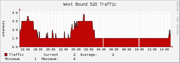
Click Graph Management, then the Add link at the top right.  Choose None from the Selected Graph Template and for the Host choose the RPi from the pull down.  We’ll set the title to “West Bound 520 Traffic”.  The next thing to set is the Vertical Label, which we’ll put “intensity”.  We’re done, so we can click Create.

Now we should have a Graph Items section added to the window.Lets start by clicking Add in that new section.  Now we can select our data source, in our case it is “WB520Data (traffic)”.  I’ll be using “C00000” for the graph color.  Next we’ll choose “AREA” as the graph type.  The only other thing I’ll set is “Traffic” in the Text Format section, which is used in the legend.

That’s it!   Now we have data being entered into Cacti…woohoo!

Here is the complete source script that Cacti uses to download, process, and read.

#!/usr/bin/python

import urllib
import os

urllib.urlretrieve("http://images.wsdot.wa.gov/nwflow/flowmaps/bridges.gif", filename="/home/pi/cacti_scripts/WSDOT_Bridges.gif")

os.system("convert -crop 4x4+238+235 +repage /home/pi/cacti_scripts/WSDOT_Bridges.gif /home/pi/cacti_scripts/cropped.gif")
os.system("convert /home/pi/cacti_scripts/cropped.gif -format %c histogram:info:/home/pi/cacti_scripts/TextFile.txt")

myfile = open("/home/pi/cacti_scripts/TextFile.txt").read().replace('\n','')
cutfile = myfile.partition('#')[2]
head, sep, tail = cutfile.partition(' ')
text_file = open("/home/pi/cacti_scripts/HEXReading.txt", "w")
text_file.write(head)
text_file.close()

if head in ('000000'):
      cactivalue = open("/home/pi/cacti_scripts/HEXReading.txt").read().replace('000000','traffic:4')
elif head in ('FF0000'):
      cactivalue = open("/home/pi/cacti_scripts/HEXReading.txt").read().replace('FF0000','traffic:3')
elif head in ('FFFF00'):
      cactivalue = open("/home/pi/cacti_scripts/HEXReading.txt").read().replace('FFFF00','traffic:2')
elif head in ('20E040'):
      cactivalue = open("/home/pi/cacti_scripts/HEXReading.txt").read().replace('20E040','traffic:1')
else:
      cactivalue = 'traffic:0'

print cactivalue

Since the grueling work is now behind us, we can move forward to the last item, which will be video from enhanced images.  We’ll do a simple normalize command in ImageMagick to create a new series of images.  Next we’ll process these to create a video stream.  Lets wrap this topic up.  Here is the command to run.

convert -normalize InputImage.jpg OutputImage.jpg

In my archive, I have around 10,000 images to process through.  It took some time to complete, 8 hours to be more precise.  Once they were done normalizing, I went ahead and processed them into a video stream.  Here are the results.  The left is the normalized images and the right are the original images.

Relations – a clearer understanding of what is

We have been briefly introduced to the subject of image processing.  The work of John Cristy at DuPont in the mid 1980s and the agreed release of it to usenet in the early 90s has given us empowerment.  We lucked out.  No one was obliged to do this work for the greater good, unlike the agreed settlement made by ATT during its monopoly breakup.

Even so, some misconceptions about image processing persist.  The name of Imagemagick is appropriate.  It is magic to the casual observer.  This give fruit to stories of how it can be used and the results it can provide.  You will see exaggerations on both sides to the capabilities and limitations of image processing.  Most of these can be discredited by observing examples that contradict the claims.  Even though the claims are more readily available than the disproving facts, you have a way to validate.  With a RPi, you can test the limits of what is possible.

If you find this subject interesting, I would suggest you read this short write up by Keith Wiley.  You may also find this example from Fred Weinhaus insightful on the whole business of image processing.  One item that I’d like to include is a Windows program that will enhance images using stacking called RegiStax.  Funny thing is ImageMagick can do the same thing with this series of commands.

convert *.jpg -evaluate-sequence median OutputFile1.jpg
convert -unsharp 1.2x1.2+5+0 OutputFile1.jpg OutputFile2.jpg
convert -normalize OutputFile2.jpg OutputFileFinal.jpg

Here is a comparison of the original next to the ImageMagick and RegiStax processed images.  You be the judge.

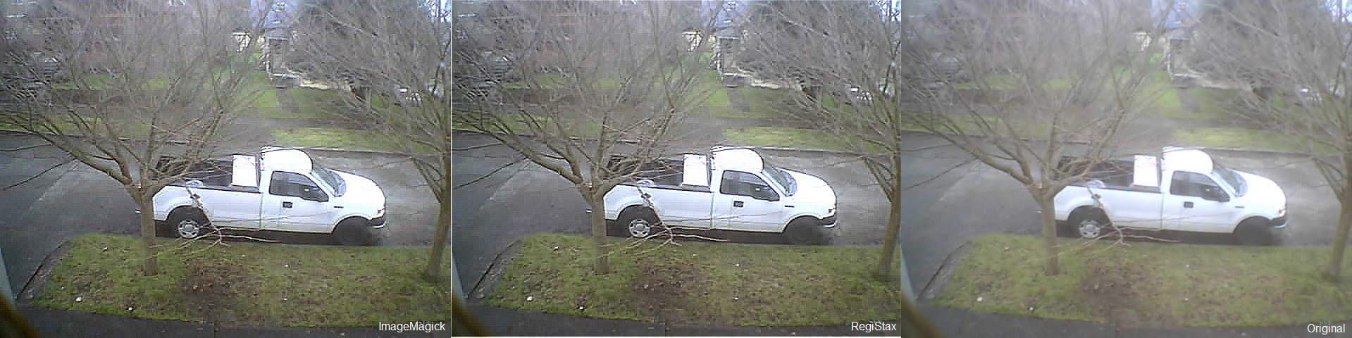
These sites were key to getting me to try it in ImageMagick.  The first explained averaging, the next explained unsharping.  I did my normalize trick at the end.

Summary – it sure can do a lot

In this post I covered some basic image processing that can be performed on the RPi using ImageMagick.  The ability of the RPi to run this processing using python is remarkable.  The data extracted from the images can be used for other applications.

We covered how to convert images into a format that allowed us to create a video from the image source.  Next we showed how image file size changes due to visual conditions.  Based on the unpredictable results of this observation method, we then covered pixel analysis.  We stepped through the process of gathering, isolating, evaluating, and plotting the results using Cacti.  Then we revisited our video processing method, but enhanced the images prior to creating the video.  Finally, we covered more enhancement options that ImageMagick offers.

In upcoming posts, we’ll cover how to crate an overlay of data on images.  This will be useful in HUD applications to display telemetry data in real time, which is a stepping stone to augmented reality.